Final Report

Motivation

We notice that a lot of smokers complain about their insurance charges. In fact, it is known that the health insurance companies stratify smokers and non-smokers and assign different insurance prices according to smoking status.

Since health insurance is vital for people’s well-being, and the cost is the main reason that stops people from buying insurance, we are interested in exploring the relationship between smoking and health insurance. To be specific, our research topic can be divided into three research questions. We would like to investigate:

If smokers tend to get insurance;
What type of insurance they prefer;
Factors that affect insurance purchasing and premiums.

Another reason that limits access to insurance is lack of information. As such, mapping of health consulting centers, health insurance carriers locations, and medicaid provider location in NYC, along with their contact information and operation hours, are also provided for readers who need more information for insurance and health advice.

Initial questions

We divide our main research topic, the relationship between smoking and health insurance, into two parts:

Smoker insurance preferences: If smokers tend to get insurance and what type of insurance they prefer
Insurance charges prediction: personal factors that affect insurance purchasing and premiums.

In the first part, insurance preferences, we first explore people’s insurance preferences and their smoking status in order to investigate if there is potential association between smoking and insurance. We also investigate some other variables that could be potential confounders or interaction factors between the relationship of smoking and insurance.

The second part, Insurance charges, assists our main research topic, since we can use the factors (age, bmi, smoker, etc) to not only explain what kind of personal characteristics would affect insurance cost, but also build a prediction model for health insurance charges. By doing such, we would gain better insights to the underlying relationship between health insurance and smoking, along with other important variables that contributes to the cost variation of insurance.

Data

Data source

Datasets for analysis

Community Health Survey Public Use Data. This dataset contains survey questions regarding smoking and health insurance. We extracted related questions from the survey for analysis.
Medical Cost Personal Dataset. This dataset sheds lights on insurance charges for different personal characteristics, such as smoking, age, Bmi, region, etc.

Datasets for mapping

Primary Care Access and Planning - Health Insurance Enrollment. This dataset is used for mapping of health consulting centers in NYC.
Medicaid Enrolled Provider Listing: This dataset is used for mapping of Medicaid provide locations in NYC.
In addition, locations of major health insurance carriers in NYC is collected manually and used to create interactive mapping of these carriers.

Data cleaning

For Community Health Survey Public Use Data, we select year 2014-2016 and variables relating to smoking, insurance, and basic health and economic status. The resulting dataset, consists of roughly 28000 participants and includes the following 12 variables:

Insurance related

insuredgateway: Whether having health insurance (1=Yes, 2=No)
insure: Type of health insurance coverage

(1 = Employer, 2 = Self-purchase,3 = Medicare, 4 = Medicaid/Family Health+, 5 = Milit/CHAMPUS/Tricare, 6 = COBRA/Other, 7 = Uninsured)

Smoking related

smoker: Smoking status (1 = Never, 2 = Current, 3 = Former)
everyday: Smoking frequency (1 = everyday smoker, 2 = casual smoker)
numberperdaya: Average cigarettes smoked per day
cost20cigarettes: Cost of 20 cigarettes (one pack)

Health and economic status

agegroup: Age groups (1 = 18-24 yrs, 2 = 25-44 yrs, 3 = 45-64 yrs, 4 = 65+ yrs)
generalhealth: Self-evaluated general health status

(1 = Excellent, 2 = Very good, 3 = Good, 4 = Fair, 5 = Poor)

sex: Participant’s sex (1 = male, 2 = female)
bmi: Participant’s BMI ($kg/m^2$)
child: Number of children the participant have: (1 = yes, 0 = no)
imputed_povertygroup: Federal poverty level(FPL) for the household

(1 = <100% FPL, 2 = 100 - <200% FPL, 3 = 200 - <400% FPL, 4 = 400 - <600% FPL, 5 = >600% FPL)

chs16 = read_sas("data/chs2016_public.sas7bdat")

chs16_filter = chs16 %>% 
  dplyr::select(agegroup,generalhealth,insuredgateway16,insure16,insured,insure5,sickadvice16,sickplace,didntgetcare16,smoker,everyday,numberperdaya,cost20cigarettes,imputed_povertygroup ,bmi,child,sex) %>% 
  mutate(year = 2016) %>% 
  dplyr::rename(insuredgateway = insuredgateway16, insure = insure16,sickadvice = sickadvice16,didntgetcare = didntgetcare16)


chs15 = read_sas("data/chs2015_public.sas7bdat")

chs15_filter = chs15 %>% 
  dplyr::select(agegroup,generalhealth,insuredgateway15,insure15,insured,insure5,sickadvice15,sickplace,didntgetcare15,smoker,everyday,numberperdaya,cost20cigarettes,imputed_povertygroup ,bmi,child,sex) %>% 
  mutate(year = 2015) %>% 
  dplyr::rename(insuredgateway = insuredgateway15, insure = insure15,sickadvice = sickadvice15,didntgetcare = didntgetcare15)


chs14 = read_sas("data/chs2014_public.sas7bdat")

chs14_filter = chs14 %>% 
  dplyr::select(agegroup,generalhealth,insuredgateway14,insure14,insured,insure5,sickadvice14,sickplace,didntgetcare14,smoker,everyday,numberperdaya,cost20cigarettes,imputed_povertygroup ,bmi,child,sex) %>% 
  mutate(year = 2014) %>% 
  dplyr::rename(insuredgateway = insuredgateway14, insure = insure14,sickadvice = sickadvice14,didntgetcare = didntgetcare14)


chs_14_16 = bind_rows(chs14_filter,chs15_filter,chs16_filter)

dataset_basic = chs_14_16 %>% 
  dplyr::select(agegroup,insure,smoker,everyday,numberperdaya,cost20cigarettes,generalhealth,imputed_povertygroup,bmi,child,sex,insuredgateway) %>% 
  mutate(numberperdaya = round(numberperdaya,1),
         imputed_povertygroup = factor(imputed_povertygroup),
         child = factor(child,levels = c(1,2)),
         sex = factor(sex),
         insure = factor(insure,levels = c(1,2,3,4,5,6,7)),
         generalhealth = factor(generalhealth,levels = c(5,4,3,2,1)),
         smoker = factor(smoker,levels = c(1,2,3)),
         everyday = factor(everyday),
         agegroup = factor(agegroup,ordered = TRUE),
         imputed_povertygroup = factor(imputed_povertygroup,levels = c(1,2,3,4,5))
         )
#write_csv(dataset_basic,"data/dataset_basic.csv")

For Medical Cost Personal Dataset, we mutate some continuous variables into factor variables

cost_df = read.csv("data/medical_cost_clean.csv") %>% 
  mutate(
    sex = as.factor(sex),
    smoker = as.factor(smoker),
    children_group = as.factor(children_group)
  )

This dataset includes the following variables

age: Age
sex: Sex (1 = male, 2 = female)
bmi: Body Mass Index
children: number of children the person has
smoker: smoking status (0 = non-smoker, 1 = smoker)
region: region in th US
charges: Insurance charges
children_group: whether or not the person has children (0 = No children, 1 = At least one child)

Exploratory analysis

dataset_basic = read_csv("data/dataset_basic.csv")

dataset_basic = read_csv("data/dataset_basic.csv") %>% 
  mutate(
         child = factor(child,levels = c(1,2),labels = c("yes","no")),
         sex = factor(sex,labels = c("male","female")),
         insure = factor(insure,levels = c(1,2,3,4,5,6,7),labels = c("Employer","Self-purchase","Medicare", "Medicaid/Family Health+", "Milit/CHAMPUS/Tricare", "COBRA/Other", "Uninsured")),
         smoker = factor(smoker,levels = c(1,2,3),labels = c("never","current","former")),
         agegroup = factor(agegroup,ordered = TRUE,labels = c("18-24yrs","25-44yrs", "45-64yrs", "65+yrs"))
         ) %>% 
  dplyr::select(insure,agegroup,smoker,bmi,child,sex)

smoke_df = read_csv("data/dataset_basic.csv") %>% 
  dplyr::select(agegroup,smoker,everyday,numberperdaya,cost20cigarettes,generalhealth,poverty_group = imputed_povertygroup,bmi,child,sex) %>% 
  drop_na(smoker) %>% 
  mutate(
         smoker_cat = case_when(
           numberperdaya <= 10 ~ 1,
           (numberperdaya > 10) & (numberperdaya <= 20) ~2,
           numberperdaya > 20 ~ 3),
         smoker_cat = factor(smoker_cat,levels = c(1,2,3),labels = c("light","normal","heavy")),

         smoker = factor(smoker,levels = c(1,2,3),labels = c("never","current","former")),
         agegroup = factor(agegroup,ordered = TRUE,labels = c("18-24yrs","25-44yrs", "45-64yrs", "65+yrs")),
         generalhealth = factor(generalhealth,levels = c(5,4,3,2,1), labels = c("Poor","Fair","Good","Very good","Excellent")),
         poverty_group = factor(poverty_group,levels = c(1,2,3,4,5),labels = c("<100% FPL","100 - <200% FPL","200 - <400% FPL","400 - <600% FPL",">600% FPL")),
         everyday = factor(everyday, levels = c(1,2), labels = c("everyday smoker", "casual smoker"))
         
         ) %>% 
  mutate(         
    smoker = fct_infreq(smoker)
)

current_smoker = smoke_df %>% filter(smoker == "current")

1. Knowledge about insurance in our dataset

Among 2941 participants in the dataset: 2582 (88%) of them are insurance holders, while 359 (12%) of them don’t have insurance cover.
Most of participants have employer-sponsored health insurance (38%), other types include Medicaid/Family Health+ (24%), Medicare (20%), Uninsured (9%), Self-purchase (6%), COBRA/Other (2%) and Milit/CHAMPUS/Tricare (1%).
Detailed introduction on each insurance type is summarized in the below table:

insurehold = read_csv("data/dataset_basic.csv") %>% 
  drop_na() %>% 
  mutate(
  insuredgateway = factor(insuredgateway, levels = c(1,2), labels = c("yes", "no"))) %>% 
  ggplot(aes(x = insuredgateway,fill = insuredgateway))+
  geom_bar()+
  theme(legend.position = "none") +
  labs(
    x = "Hold status of insurance",
    y = "Number of participants",
    title = "Holding status of insurace among participants")

insuretype = dataset_basic %>% 
  drop_na() %>% 
  mutate(insure = fct_infreq(insure)) %>% 
  ggplot(aes(x = insure,fill = insure))+
  geom_bar()+
  theme(legend.position = "none") +
  theme(plot.title = element_text(hjust = 0.5)) +
  labs(
    x = "Insurance type",
    y = "Number of holders",
    title = "Number of holders\nin each insurance type") + 
  coord_flip()

#| my-chunkhaha, echo = FALSE, fig.width = 8,
insurehold + insuretype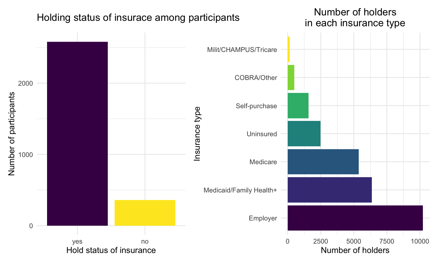

insur_type <- c("Employer", "Medicare", "Milit/CHAMPUS", "Uninsured", "Self-purchased", "Medicaid/Family Health+", "COBRA/other")

insur_meaning <- c("Employer-sponsored health insurance is a health insurance selected and purchased by your employer and offered to eligible employees and their dependents.",
                   "Medicare is federal health insurance for people 65 or older, some younger people with disabilities, people with End-Stage Renal Disease",
                   "Health Care progam for military",
                   "Not insured",
                   "Insurance purchased by individual choice",
                   "Medicaid/health insurance program for adults who are aged 19 to 64 who have income too high to qualify for Medicaid",
                   "Consolidated Omnibus Budget Reconciliation Act, which gives some employees the ability to continue health insurance coverage after leaving employment, or other types of insurance.")

insur <- data.frame(insur_type, insur_meaning) %>% 
  dplyr::rename(
    "Insurance type" = insur_type,
    "Insurance type meaning" = insur_meaning
  )
knitr::kable(insur)

Insurance type	Insurance type meaning
Employer	Employer-sponsored health insurance is a health insurance selected and purchased by your employer and offered to eligible employees and their dependents.
Medicare	Medicare is federal health insurance for people 65 or older, some younger people with disabilities, people with End-Stage Renal Disease
Milit/CHAMPUS	Health Care progam for military
Uninsured	Not insured
Self-purchased	Insurance purchased by individual choice
Medicaid/Family Health+	Medicaid/health insurance program for adults who are aged 19 to 64 who have income too high to qualify for Medicaid
COBRA/other	Consolidated Omnibus Budget Reconciliation Act, which gives some employees the ability to continue health insurance coverage after leaving employment, or other types of insurance.

2. Knowledge regarding smoking in our dataset

Here we conduct some explorations focusing on smoking information in our data. Click on each tab to see different dimensions of smoking data.

Smoking status

Age distribution

smokegroup_count = smoke_df %>% 
  drop_na(smoker) %>% 
  dplyr::group_by(smoker) %>% 
  dplyr::summarize(
    smokegroup_count = n()) %>% 
  pull()

smoke_df %>% 
  drop_na(agegroup) %>% 
  dplyr::group_by(agegroup,smoker) %>% 
  dplyr::summarize(
    age_count = n()) %>% 
  mutate(smokegroup_count = smokegroup_count,
         age_percent = age_count/smokegroup_count) %>% 
  ggplot(aes(x = smoker, y = age_percent, fill = agegroup)) + 
  geom_bar(stat = "identity",position = "dodge") +
    labs(
      x = 'Smoking status',
      y = 'Proportion',
      title = 'Age distribution among people in different smoking status',
      fill = "Age Group" )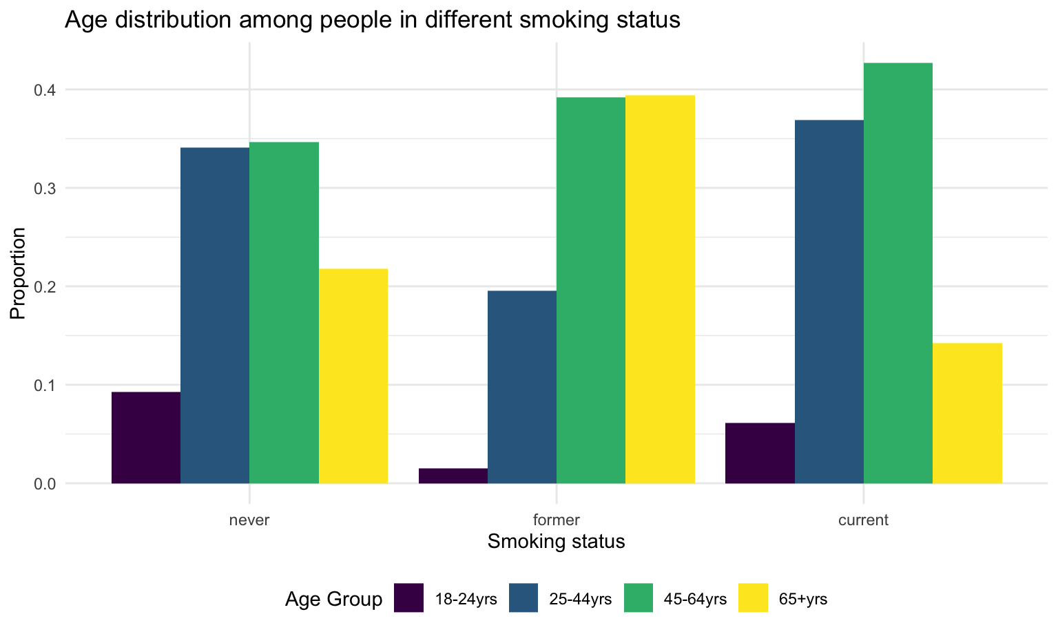

There are a total 3652 (12%) current smokers, 6167 (21%) former smokers, and 18693 (66%) people never smoked among all the participants. Most current smokers falls in age 25 to 64 (80%). 84% of the paticipants in age 18-24 filter have never smoked.

Health self-evaluation

smoke_df %>% 
  drop_na(generalhealth) %>% 
  dplyr::group_by(generalhealth,smoker) %>% 
  dplyr::summarize(
    count = n())%>% 
  mutate(smokegroup_count = smokegroup_count,
         health_percent = count/smokegroup_count)%>% 
  ggplot(aes(x = smoker, y = health_percent, fill = generalhealth)) + 
  geom_bar(stat = "identity",position = "dodge") +
    labs(
      x = 'Smoking status',
      y = 'Health self-evaluation \n(% in each types of smoker)',
      title = 'Self-evaluation of health conditions among people in different smoking status\n(% in each types of smoker)',
      fill = "Health status" )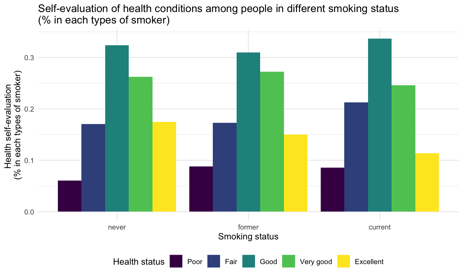

Compare with other groups, current smokers have lowest proportion of excellent health status(self-evaluated).

Poverty status

smoke_df %>% 
  drop_na(poverty_group) %>% 
  dplyr::group_by(poverty_group,smoker) %>% 
  dplyr::summarize(
    count = n()
  ) %>% 
  mutate(
    smokegroup_count = smokegroup_count,
    poverty_percent = count/smokegroup_count) %>% 
  ggplot(aes(x = smoker, y = poverty_percent, fill = poverty_group)) + 
  geom_bar(stat = "identity",position = "dodge") +
    labs(
      x = 'Smoking status',
      y = 'Poverty groups\n(% in each types of smoker)',
      title = 'Poverty groups (% in each types of smoker)',
      fill = "Poverty Group" )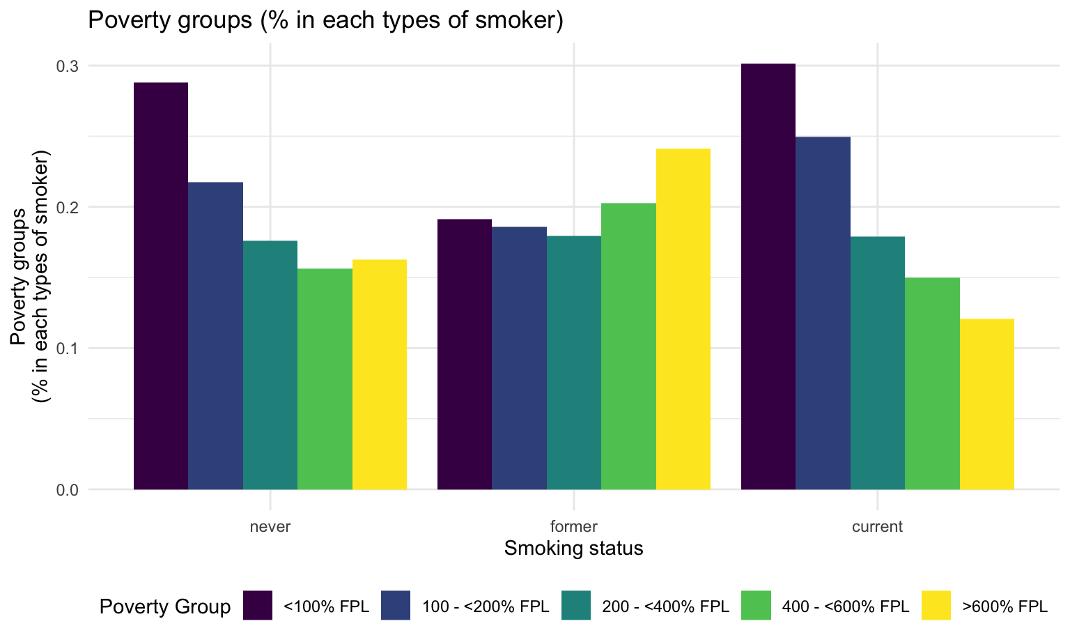

Comparing to other groups, current smokers have the largest proportion of people who are <100% FPL, which means unsatisfactory financial status. They also have the least proportion of people who are >600 FPL, indicating atisfactory financial status.

BMI

smoke_df %>% 
  drop_na(bmi,smoker) %>% 
  ggplot(aes(x = smoker, y = bmi,fill = smoker)) + 
  geom_boxplot() +
  ylim(0,50)+
    labs(
      x = 'Smoking status',
      y = 'BMI (kg/m^2)',
      title = 'The distribution of bmi among people in different smoking status')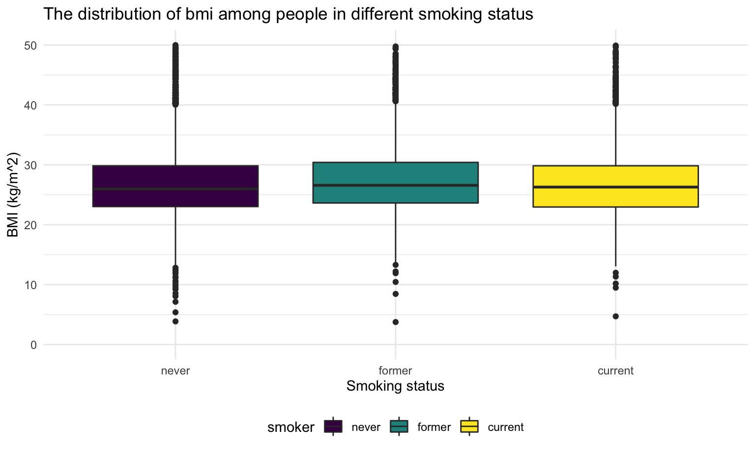

There’s no significant difference of participants BMI in different smoking status.

Current smokers

Next, we focus on the current smokers and look at there smoking intensity, frequency and cost, as well as their BMI index.

Smoking intensity and frequency

type = current_smoker %>%
  ggplot(aes(x = smoker_cat, fill = everyday))+
  geom_histogram(stat="count") +
    labs(
      x = 'Smoking intensity',
      y = 'Number of current smokers',
      title = 'Smoking intensity of current smokers')+
  theme(legend.position = "none")

consumption = current_smoker %>% 
  ggplot(aes(x = numberperdaya, fill = everyday)) + 
  geom_histogram()+
  xlim(0,30)+
  labs(
    x = "Average number of cigarattes smoked per day",
    y = "Number of current smokers",
    title = "Average number of cigarattes\nsmoked per day",
    fill = "Smoking frequency"
       )+
  theme(legend.position = "right")

#| my-chunkn1, echo = FALSE, fig.width = 8,
type + consumption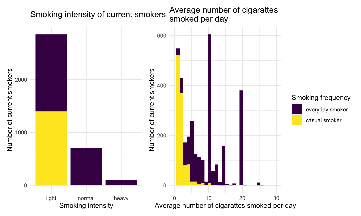

Most of the current smokers are light smokers. Among those light smokers, nearly half of them smoke everyday, while normal and heavy smokers are more likely to smoke everyday. Casual smokers tend to consume less cigarette than everyday smokers.

BMI

current_smoker %>% 
  ggplot(aes(x = smoker_cat, y = bmi, fill = smoker_cat))+
  geom_boxplot() +
  theme(plot.title = element_text(hjust = 0.5)) +
  ylim(0,50)+
  #facet_grid(.~smoker_cat,scales = "free") +
    labs(
      x = 'Smoking intensity',
      y = 'BMI (kg/m^2)',
      title = 'BMI among current smokers with different smoking intensity',
      color = "Smoking intensity")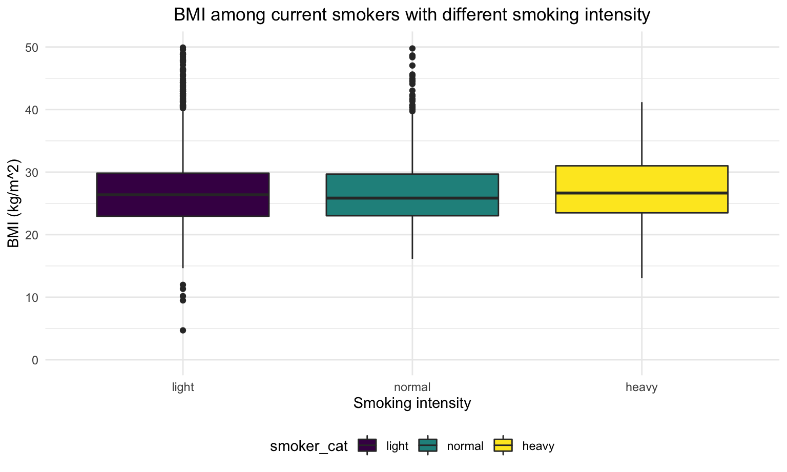

For heavy smokers, their BMI are slightly higher than light smokers and normal smokers.

Cost on smoke

current_smoker %>% 
  ggplot(aes(x = numberperdaya, y = cost20cigarettes,color = everyday))+
  geom_point(alpha = .5,size = 3) +
  xlim(0,50)+
  ylim(0,40)+
  theme(plot.title = element_text(hjust = 0.5)) +
  #facet_grid(.~smoker_cat,scales = "free") +
    labs(
      x = 'Number of cigrattes consumed everyday',
      y = 'Cost of every 20 (one pack) cigrattes',
      title = 'Cost of every 20 (one pack) cigrattes\nfor number of cigrattes consumed everyday',
      color = "Smoking frequency")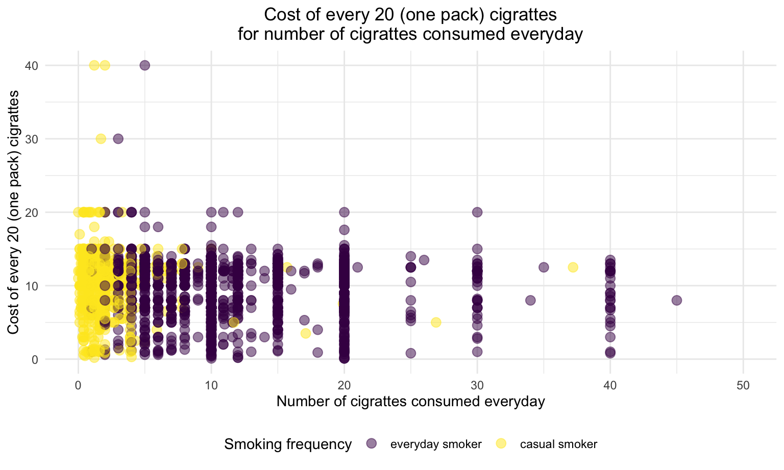

Regardless of smoking frequency and smoking intensity, the cost of each pack of cigarette are even distributed within $0 to $20

3. Explore relationship between insurance and target variables

In this step, we want to explore more about the relationship between insurance and key variables, including smoking, age, have children or not and BMI. We start by plotting distribution graphs to see the pattern between each groups. And then we conduct statistical tests to evaluate the association and similarity between them.

Distributions

Smoking

#| my-chunkn, echo = FALSE, fig.width = 10,
analyse_smoke_sum = 
  dataset_basic %>%
  drop_na(smoker,insure) %>% 
  dplyr::group_by(smoker,insure) %>% 
  dplyr::summarize(n = n()) %>% 
  mutate(insure = fct_reorder(insure,n)) %>% 
  ungroup() %>% 
  dplyr::group_by(smoker) %>% 
  dplyr::summarize(sum = sum(n)) %>% 
  pull()

analyse_smoke_insurancetype = dataset_basic %>%
  drop_na(smoker,insure) %>% 
  dplyr::group_by(smoker,insure) %>% 
  dplyr::summarize(n = n()) %>% 
  mutate(insure = fct_reorder(insure,n)
         ) 

analyse_smoke_insurancetype$sum = rep(analyse_smoke_sum, each = 7)

analyse_smoke_insurancetype =
  analyse_smoke_insurancetype %>% 
  mutate(
    freq = n/sum
  )

uninsure = analyse_smoke_insurancetype %>% 
  mutate(insure = ifelse(insure == "Uninsured", "Uninsured", "Insured"))
  
  

smoke_plot1 = analyse_smoke_insurancetype %>% 
  ggplot(aes(x =smoker , y = freq, fill = insure)) + 
  geom_bar(stat = "identity",position = "dodge") +
    labs(
      x = 'smoking status ',
      y = 'proportion',
      title = 'The proportion of insurance in different smoking group ',
      fill = "Insurance type")+
  theme(legend.position = "right")

smoke_plot2 = uninsure %>% 
  ggplot(aes(x =smoker , y = freq, fill = insure)) + 
  geom_bar(stat = "identity",position = "dodge") +
    labs(
      x = 'smoking status ',
      y = 'proportion',
      title = 'The proportion of insurance\nin different smoking group ',
      fill = "Insurance status")

smoke_plot2 + smoke_plot1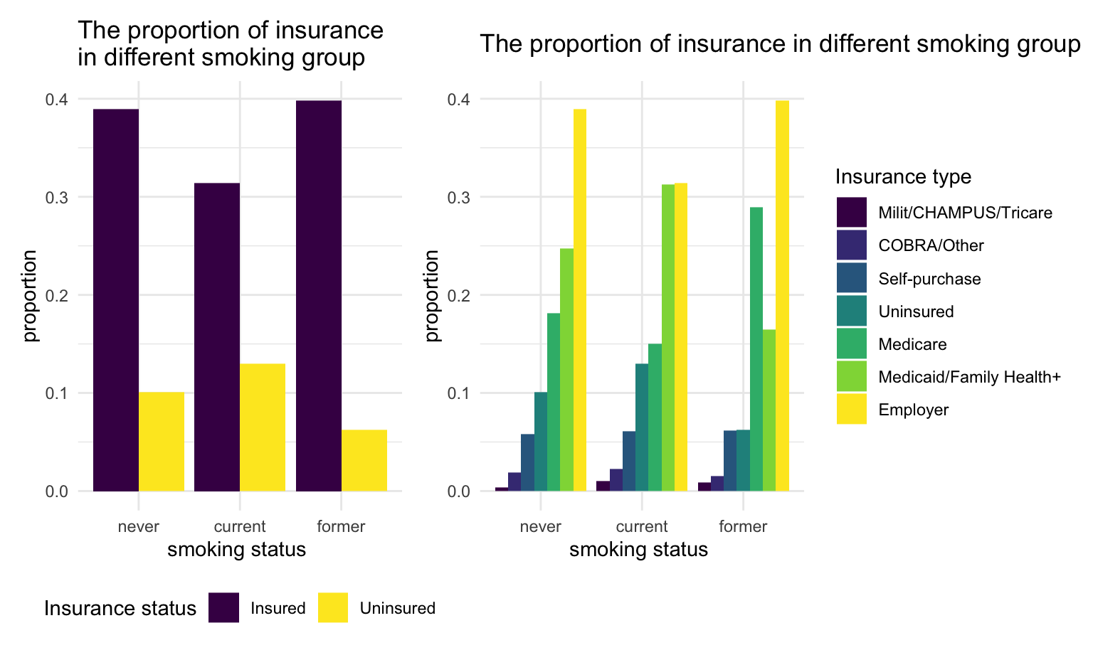

We found that, current smokers have the highest uninsured proportion comparing to other groups.

Regardless of the smoking status, most people tend to get employer insurance. For former smokers, a larger proportion of them get the medicare insurance compare to people who never smoke or currently smoke.

Age

#| my-chunkn2, echo = FALSE, fig.width = 10,
analyse_agegroup_sum = 
  dataset_basic %>%
  drop_na(agegroup,insure) %>% 
  dplyr::group_by(agegroup,insure) %>% 
  dplyr::summarize(n = n()) %>% 
  mutate(insure = fct_reorder(insure,n)) %>% 
  ungroup() %>% 
  dplyr::group_by(agegroup) %>% 
  dplyr::summarize(sum = sum(n)) %>% 
  pull()

analyse_agegroup_insurancetype = dataset_basic %>%
  drop_na(agegroup,insure) %>% 
  dplyr::group_by(agegroup,insure) %>% 
  dplyr::summarize(n = n()) %>% 
  mutate(insure = fct_reorder(insure,n)
         ) 

analyse_agegroup_insurancetype$sum = rep(analyse_agegroup_sum, each = 7)

analyse_agegroup_insurancetype =
  analyse_agegroup_insurancetype %>% 
  mutate(
    freq = n/sum
  )

uninsure = analyse_agegroup_insurancetype %>% 
  mutate(insure = ifelse(insure == "Uninsured", "Uninsured", "Insuredd"))
  
  

agegroup_plot1 = analyse_agegroup_insurancetype %>% 
  ggplot(aes(x = agegroup, y = freq, fill = insure  )) + 
  geom_bar(stat = "identity",position = "dodge") +
    labs(
      x = 'agegroup',
      y = 'proportion',
      title = 'The distribution of insurance type in differnt age groups') +
  theme(legend.position = "right")

agegroup_plot2 = uninsure %>% 
  ggplot(aes(x =agegroup , y = freq, fill = insure)) + 
  geom_bar(stat = "identity",position = "dodge") +
    labs(
      x = 'agegroup',
      y = 'proportion',
      title = 'The proportion of insurance\nin different age group ',
      fill = "Insurance status")

agegroup_plot2 + agegroup_plot1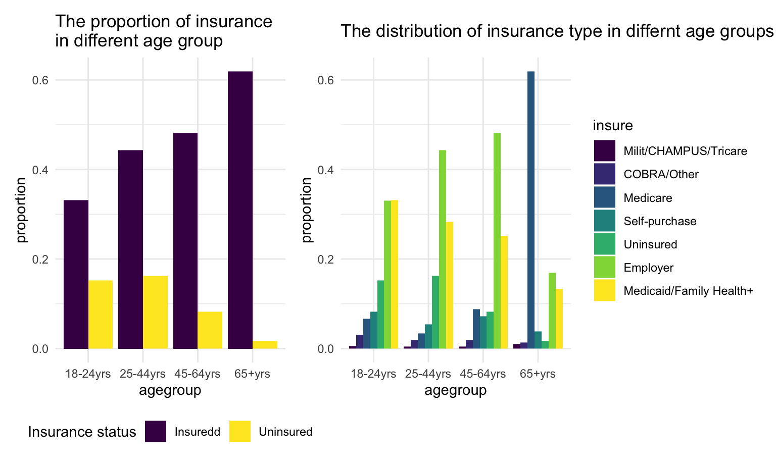

For person younger than 65 years old, people tend to get insurance as age increase. Specifically, for those age in the range of 25-64 years old, high proportion of them get employer insurance since they are in working age.

For person older than 65 years old, most of them get Medicare since Medicare is only provided for people above 65 years old.

Have children or not

#| my-chunkn3, echo = FALSE, fig.width = 10,
analyse_child_sum = 
  dataset_basic %>%
  drop_na(child,insure) %>% 
  dplyr::group_by(child,insure) %>% 
  dplyr::summarize(n = n()) %>% 
  mutate(insure = fct_reorder(insure,n)) %>% 
  ungroup() %>% 
  dplyr::group_by(child) %>% 
  dplyr::summarize(sum = sum(n)) %>% 
  pull()

analyse_child_insurancetype = dataset_basic %>%
  drop_na(child,insure) %>% 
  dplyr::group_by(child,insure) %>% 
  dplyr::summarize(n = n()) %>% 
  mutate(insure = fct_reorder(insure,n)
         ) 

analyse_child_insurancetype$sum = rep(analyse_child_sum, each = 7)

analyse_child_insurancetype =
  analyse_child_insurancetype %>% 
  mutate(
    freq = n/sum
  )

uninsure = analyse_child_insurancetype %>% 
  mutate(insure = ifelse(insure == "Uninsured", "Uninsured", "Insured"))
  
  

child_plot1 = analyse_child_insurancetype %>% 
  ggplot(aes(x = child, y = freq, fill = insure  )) + 
  geom_bar(stat = "identity",position = "dodge") +
    labs(
      x = 'have children or not',
      y = 'proportion',
      title = 'Distribution of insurance type in groups\nof people with or without children') +
  theme(legend.position = "right")

child_plot2 = uninsure %>% 
  ggplot(aes(x =child , y = freq, fill = insure)) + 
  geom_bar(stat = "identity",position = "dodge") +
    labs(
      x = 'have children or not',
      y = 'proportion',
      title = 'Proportion of insurance in groups\nof people with or without children',
      fill = "Insurance status")

child_plot2 + child_plot1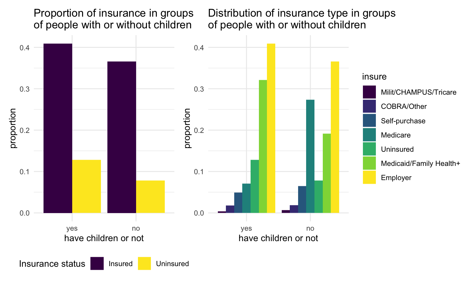

We found that for those without children, a larger proportion of them get Medicare comparing to those with children.

BMI

analyse_bmi_insurancetype = 
  dataset_basic %>%
  drop_na(bmi,insure) 
  
uninsure_bmi = analyse_bmi_insurancetype %>% 
  mutate(insure = ifelse(insure == "Uninsured", "Uninsured", "Insured"))
  
bmi_plot1 = 
  analyse_bmi_insurancetype %>% 
  ggplot(aes(x = insure, y = bmi,fill = insure)) + 
  geom_boxplot(alpha = 0.6) +
    theme(legend.position = "none") +
    scale_fill_brewer(palette = "Dark2") +
    labs(
      x = 'insurance',
      y = 'bmi',
      title = 'The distribution of bmi in groups\nhaving different insurance type') +
  coord_flip()


bmi_plot2 = 
  uninsure_bmi %>% 
  ggplot(aes(x = insure , y = bmi, fill = insure)) + 
  geom_boxplot(alpha = 0.6) +
    theme(legend.position = "none") +
    scale_fill_brewer(palette = "Dark2") +
    labs(
      x = 'have insurance or not',
      y = 'bmi',
      title = 'The distribution of bmi in groups\nhaving insurance or not') +
  coord_flip()

bmi_plot2 + bmi_plot1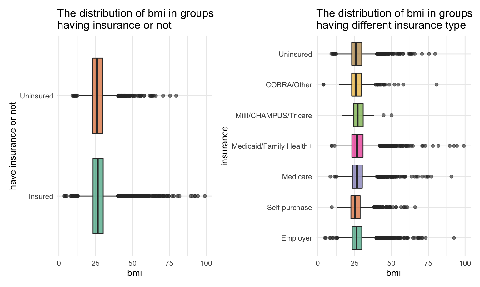

We did not observe significant difference between each group.

Statistical test

From the plots, we could find out many patterns about the relations between insurance status and smoking age and have children or not. To further validate the uncertain association between insurance type and other key factors as well as between insurance status and BMI, we conduct several statistical tests as follows.

Smoking

Chi-quare test between insurance type and smoking

$H_0$ : insurance type and smoking are independent, there is no relationship between the two categorical variables.

$H_1$ : insurance type and smoking are dependent, there is a relationship between the two categorical variables.

Test result:

dat = 
  dataset_basic %>%
  drop_na(smoker,insure)

#| my-chunk1, echo = FALSE, fig.width = 8,

# plot
ggbarstats(
  data = dat,
  x = smoker,
  y = insure,
  title = "Chi-quare test between insurance type and smoking"
) +
  labs(caption = NULL) +
  theme(
    axis.text.x = element_text(angle = 90, vjust = .5, hjust = 1)
  )

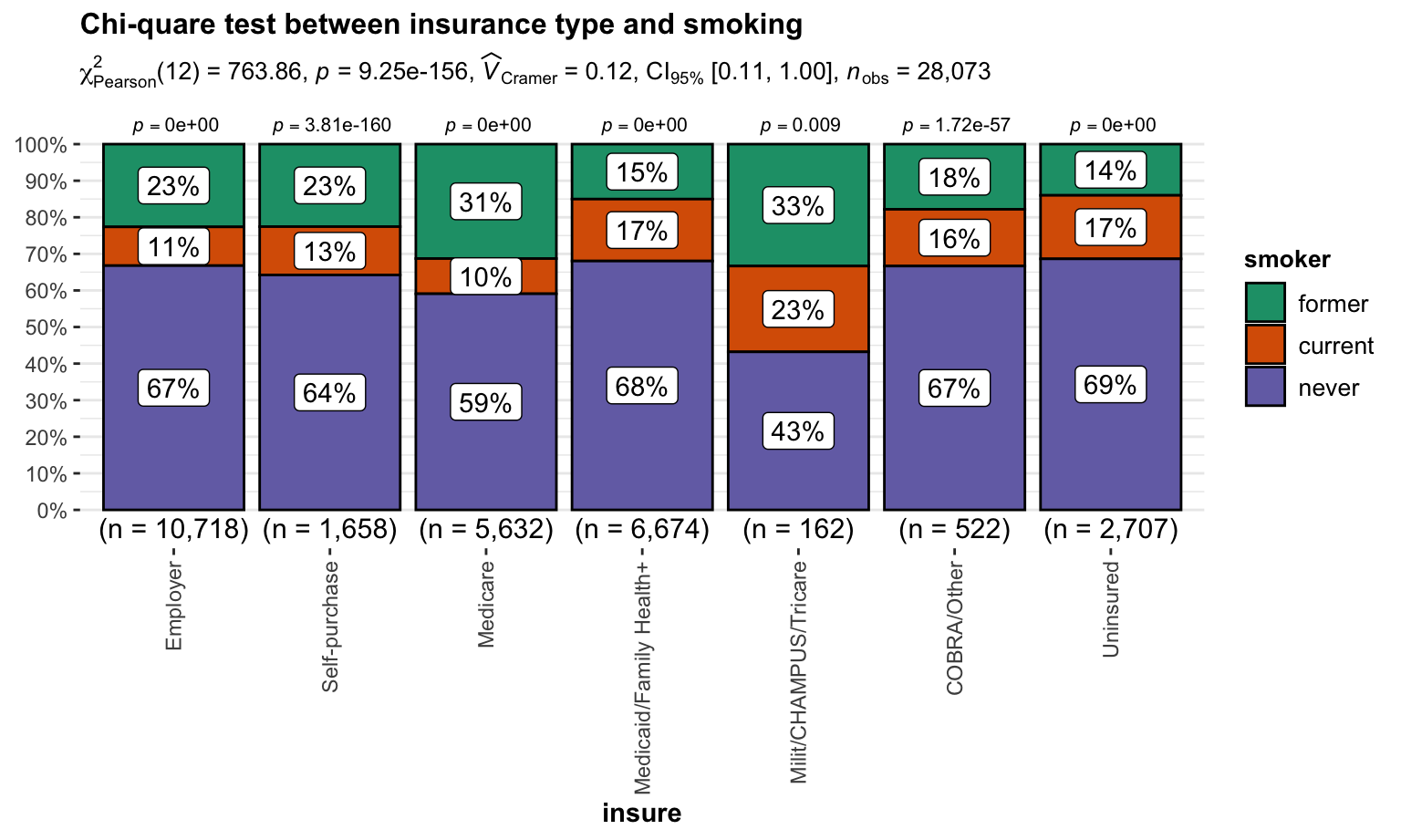
We reject $H_0$ and then conclude that insurance type and smoking are dependent.

Age

Chi-quare test between insurance type and age

$H_0$ : insurance type and age are independent, there is no relationship between the two categorical variables.

$H_1$ : insurance type and age are dependent, there is a relationship between the two categorical variables.

Test result:

dat = 
  dataset_basic %>%
  drop_na(agegroup,insure)

#| my-chunk2, echo = FALSE, fig.width = 8,
ggbarstats(
  data = dat,
  x = smoker,
  y = insure,
  title = "Chi-quare test result between insurance type and age"
) +
  labs(caption = NULL) +
  theme(
    axis.text.x = element_text(angle = 90, vjust = .5, hjust = 1)
  )

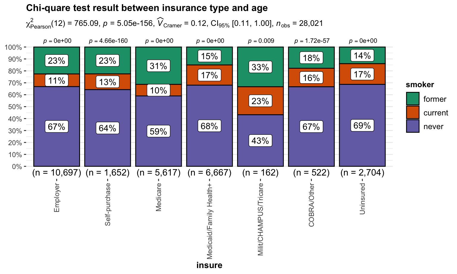
We reject $H_0$ and then conclude that insurance type and age are dependent.

Have children or not

Chi-quare test between insurance type and children

$H_0$ : insurance type and have children or not are independent, there is no relationship between the two categorical variables.

$H_1$ : insurance type and have children or not are dependent, there is a relationship between the two categorical variables.

Test result:

#test_data_smoke_insurancetype = analyse_smoke_insurancetype %>% 
#  pivot_wider(
#  names_from = "Insured", 
#  values_from = "n")

#test_data_smoke_insurancetype %>% knitr::kable()
#chisq.test(test_data_smoke_insurancetype[-1])

dat = 
  dataset_basic %>%
  drop_na(child,insure)

#| my-chunk3, echo = FALSE, fig.width = 8,

ggbarstats(
  data = dat,
  x = child,
  y = insure,
  title = "Chi-quare test between insurance type and children"
) +
  labs(caption = NULL) +
  theme(
    axis.text.x = element_text(angle = 90, vjust = .5, hjust = 1)
  )

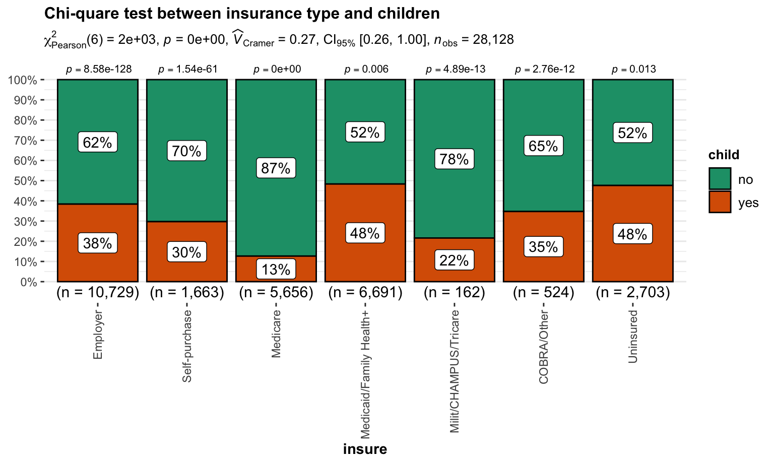
We reject $H_0$ and then conclude that insurance type and children are dependent.

BMI

ANOVA test between insurance status and BMI

$H_0$ : The mean of BMI in groups with or without insurance are the same

$H_1$ : The means of BMI in groups with or without insurance are different

Test result:

#| my-chunk61, echo = FALSE, fig.width = 10,fig.height = 8
anova = aov( bmi ~insure, data = uninsure_bmi)
anova %>% 
  broom::tidy() %>% 
  knitr::kable()

term	df	sumsq	meansq	statistic	p.value
insure	1	5.716116e+01	57.16116	1.529227	0.2162393
Residuals	26922	1.006321e+06	37.37912	NA	NA

According to the ANOVA test, we can not reject $H_0$ and conclude the mean of BMI in each insurance type groups are the same.

ANOVA test between insurance type and BMI

$H_0$ : The mean of BMI in each insurance type groups are the same

$H_1$ : At least two means of BMI in all insurance type groups are different

Test result:

#| my-chunk62, echo = FALSE, fig.width = 10,fig.height = 8
anova = aov( bmi ~insure, data = analyse_bmi_insurancetype)
anova %>% 
  broom::tidy() %>% 
  knitr::kable()

term	df	sumsq	meansq	statistic	p.value
insure	6	2435.492	405.9154	10.88312	0
Residuals	26917	1003942.322	37.2977	NA	NA

Tukey_comp = TukeyHSD(anova)

par(mar = c(2, 18, 2, 2))
plot(Tukey_comp,las = 1,
     cex.axis = 0.8)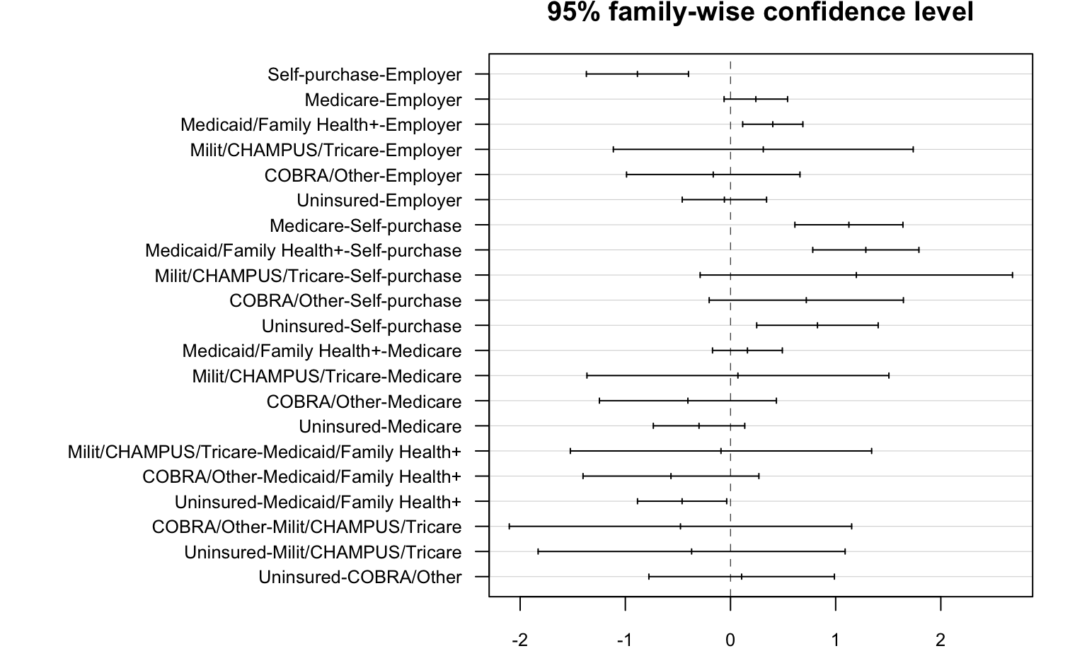

Additional analysis

In order to assists our main research topic, the relationship between smoking and health insurance, we would like to investigate the amount of insurance price change due to smoking, along with other personal factors such age, sex, weight and whether or not having children. A prediction model is build to analyse this question.

A snapshot of the vairables

We selected the following variable for modeling. Detailed information are in the table below:

var <- c("smoker", "children_group", "sex", "age", "bmi", "charges")

var_meaning <- c("0 = non-smoker, 1 = smoker", "0 = No children, 1 = Have at least 1 child", "1 = male, 2 = female", "Age range from 18 to 63", "Body mass index range from 15.96 to 53.13", "Cost of health insurance")

var_info <- data.frame(var, var_meaning) %>% 
  dplyr::rename(
    "Variable name" = var,
    "Variable information" = var_meaning
  )
knitr::kable(var_info)

Variable name	Variable information
smoker	0 = non-smoker, 1 = smoker
children_group	0 = No children, 1 = Have at least 1 child
sex	1 = male, 2 = female
age	Age range from 18 to 63
bmi	Body mass index range from 15.96 to 53.13
charges	Cost of health insurance

1. Relationship between each variables and charge of insurance

Smoker and insurance charges

cost_df_smoker = 
  cost_df %>%
  mutate(
    smoker = fct_recode(
      smoker,
      "Smoker" = "1",
      "Non smoker" = "0"
      ))
    
smoker_plotly <- cost_df_smoker %>% 
  plot_ly(
    x = ~smoker,
    y = ~charges,
    split = ~smoker,
    type = 'violin',
    box = list(
      visible = T
    ),
    meanline = list(
      visible = T
    )
  ) 

smoker_plotly <- smoker_plotly %>%
  layout(
    xaxis = list(
      title = "smokeing status"
    ),
    yaxis = list(
      title = "Insurance charges",
      zeroline = F
    ),
    legend=list(title=list(text='<b> Smokering Status </b>'))
  )

smoker_plotly

Having children and insurance charges

cost_df_child = 
  cost_df %>%
  mutate(
    children_group = fct_recode(
      children_group,
      "Having at least one child" = "1",
      "No children" = "0"
      ))
    
child_plotly <- cost_df_child %>% 
  plot_ly(
    x = ~children_group,
    y = ~charges,
    split = ~children_group,
    type = 'violin',
    box = list(
      visible = T
    ),
    meanline = list(
      visible = T
    )
  ) 

child_plotly <- child_plotly %>%
  layout(
    xaxis = list(
      title = "Whether or not having children"
    ),
    yaxis = list(
      title = "Insurance charges",
      zeroline = F
    ),
    legend=list(title=list(text='<b> Whether or not having children </b>'))
  )

child_plotly

Gender and insurance charges

cost_df_sex = 
  cost_df %>%
  mutate(
    sex = fct_recode(
      sex,
      "Male" = "1",
      "Female" = "2"
      ))
    
sex_plotly <- cost_df_sex %>% 
  plot_ly(
    x = ~sex,
    y = ~charges,
    split = ~sex,
    type = 'violin',
    box = list(
      visible = T
    ),
    meanline = list(
      visible = T
    )
  ) 

sex_plotly <- sex_plotly %>%
  layout(
    xaxis = list(
      title = "Gender"
    ),
    yaxis = list(
      title = "Insurance charges",
      zeroline = F
    ) ,
    legend=list(title=list(text='<b> Gender </b>'))
  )

sex_plotly

Age and insurance charges

age_fit <- lm(charges ~ age, data = cost_df)


age_plotly <- plot_ly(
  cost_df, 
  x = ~age, 
  y = ~charges,
  color = ~age,
  size = ~age,
  name = ""
  ) %>% 
  add_markers(y = ~charges) %>% 
  add_lines(x = ~age, y = fitted(age_fit), color = "") %>% 
  layout(
   showlegend = FALSE
  )


age_plotly

BMI and insurance charges

bmi_fit <- lm(charges ~ bmi, data = cost_df)


bmi_plotly <- plot_ly(
  cost_df, 
  x = ~bmi, 
  y = ~charges,
  color = ~bmi, 
  size = ~bmi,
  name = ""
  ) %>% 
  add_markers(y = ~charges) %>% 
  add_lines(x = ~bmi, y = fitted(bmi_fit), color = "") %>% 
  layout(showlegend = FALSE)


bmi_plotly

From the five plots above, we can tell that smoking, age, and bmi significantly affect charge of insurance. The relationship between charges and gender or having children is unclear. Further analysis will be carried below to illustrate their relationships.

2. Model selection

Correlation plot

cost_df_cor = cost_df %>% 
  dplyr::select(age, sex, bmi, smoker, charges, children_group)

model.matrix(~0+., data = cost_df_cor) %>% 
  cor(use="pairwise.complete.obs") %>% 
  ggcorrplot(show.diag = F, type="lower", lab=TRUE, lab_size=2)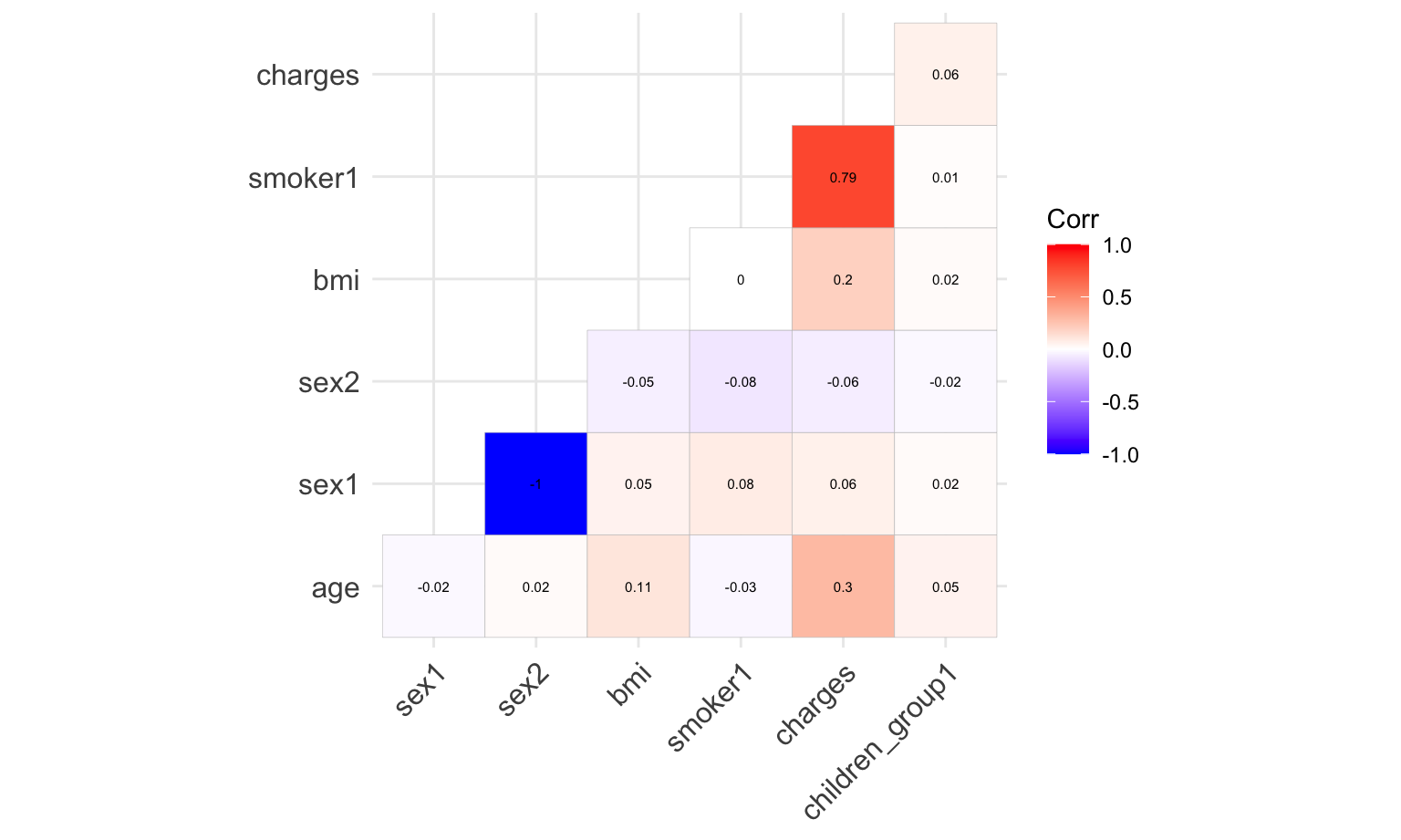

There is no collinearity between any of the variables. Therefore, no need to adjust variable for model building. In addition, smoking seems to be the highest correlated variable to charges among other variables.

Fit regression using all predictors

model <- lm(charges ~ smoker + children_group + sex + age + bmi, data = cost_df)
summary(model)%>% 
  broom::tidy() %>% 
  knitr::kable()

term	estimate	std.error	statistic	p.value
(Intercept)	-12225.0034	970.40293	-12.5978633	0.0000000
smoker1	23822.2843	413.01074	57.6795754	0.0000000
children_group1	992.5886	336.10888	2.9531757	0.0032004
sex2	123.6608	333.73639	0.3705345	0.7110432
age	257.8266	11.91998	21.6297878	0.0000000
bmi	322.2230	27.45121	11.7380271	0.0000000

The model building result shows that sex is not a significant variable with p-value < 0.05. Therefore, when we do the stepwise regression, we would likely to remove the variable of sex.

Stepwise regression

step = step(model, direction='both')

summary(step)%>% 
  broom::tidy() %>% 
  knitr::kable()

term	estimate	std.error	statistic	p.value
(Intercept)	-12149.6071	948.52261	-12.808980	0.000000
smoker1	23810.7572	411.70416	57.834629	0.000000
children_group1	990.7412	335.96313	2.948958	0.003244
age	257.9366	11.91243	21.652729	0.000000
bmi	321.7303	27.41011	11.737652	0.000000

The stepwise regression process confirms that sex is not significant variable. Therefore we remove sex variable and retain all other variables for prediction model.

Final model with significant variables

model1 <- lm(charges ~ smoker + children_group + age + bmi, data = cost_df)
summary(model1) %>% 
  broom::tidy() %>% 
  knitr::kable()

term	estimate	std.error	statistic	p.value
(Intercept)	-12149.6071	948.52261	-12.808980	0.000000
smoker1	23810.7572	411.70416	57.834629	0.000000
children_group1	990.7412	335.96313	2.948958	0.003244
age	257.9366	11.91243	21.652729	0.000000
bmi	321.7303	27.41011	11.737652	0.000000

3. Model diagnostic

par(mfrow = c(2,2))
plot(model1)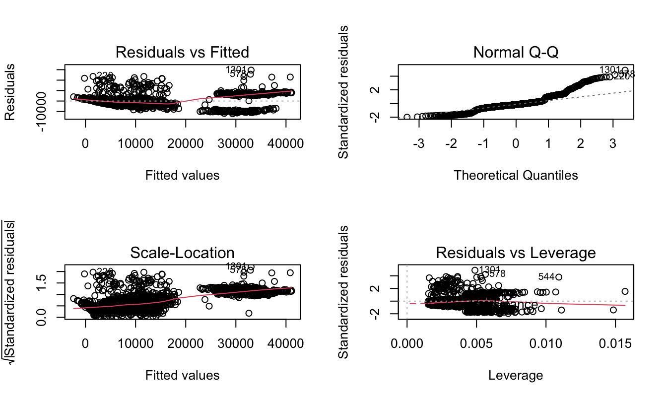

The graph above did not show homoscedasticity of residual. Therefore, we need to transform the model.

4. Model transformation

Box-Cox Transformation

par(mfrow = c(1,2))

boxcox(model1, lambda = seq(-3, 3, by = 0.25)) 

plot(model1, which = 4) # remove 544, 578, 1301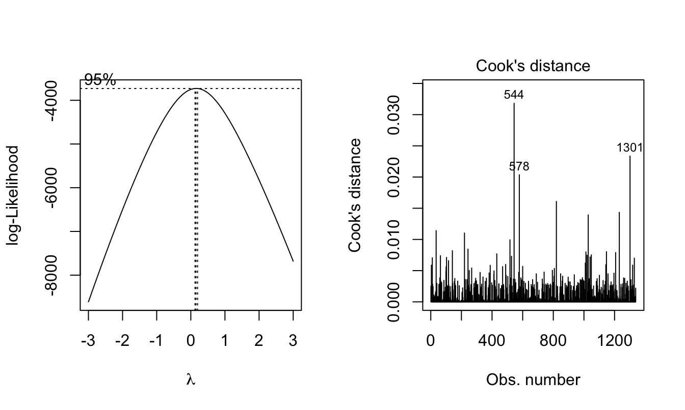

cost_df_out = cost_df[-c(544,578, 1301),]

Since lamda = 0, try natural log transformation.

Before transformation, remove outliers first

The outliers are rows 544, 578, 1301. Following model building will use dataset without these outliers.

Transform charges to ln(charges)

#summary(cost_df_out)
cost_df_log = cost_df_out %>% 
  mutate(
    Lncharges = log(charges)
  ) 

# fit multivariate model with log transform
model_log = lm(Lncharges ~ smoker + children_group + age + bmi, data = cost_df_log) 
summary(model_log) %>% 
  broom::tidy() %>% 
  knitr::kable()

term	estimate	std.error	statistic	p.value
(Intercept)	6.9709701	0.0706776	98.630532	0e+00
smoker1	1.5370576	0.0307293	50.019359	0e+00
children_group1	0.2263090	0.0250004	9.052215	0e+00
age	0.0347807	0.0008857	39.268460	0e+00
bmi	0.0103985	0.0020435	5.088614	4e-07

Above table shows the estimates for each variables when charges is transformed to In(charges).

Diagnostic for transformed model

par(mfrow = c(1,2))

boxcox(model_log)

plot(model_log, which = 1)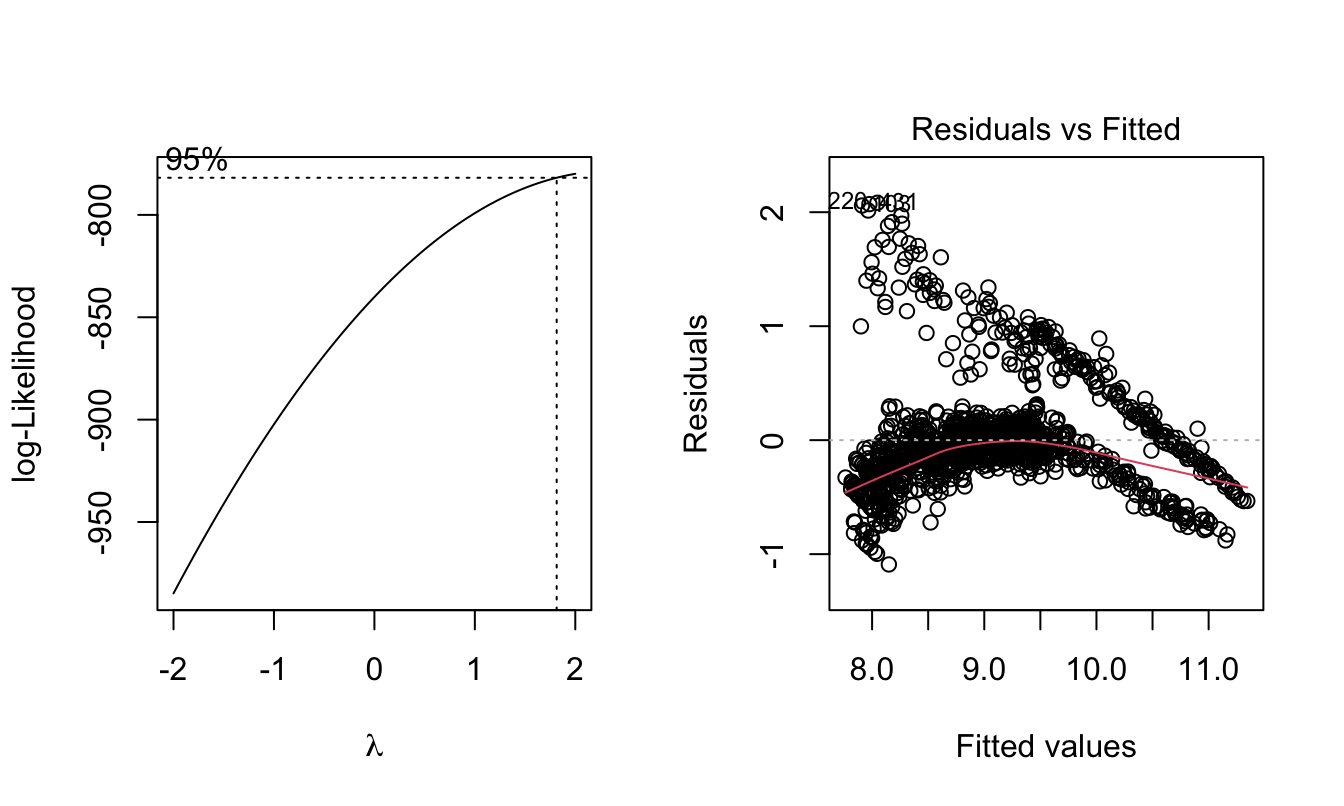

Lamda is near 1 now, and the residual distribution improved from un-transformed data. We conclude this model is acceptable.

Final model

summary(model_log) %>% 
  broom::tidy() %>% 
  knitr::kable()

term	estimate	std.error	statistic	p.value
(Intercept)	6.9709701	0.0706776	98.630532	0e+00
smoker1	1.5370576	0.0307293	50.019359	0e+00
children_group1	0.2263090	0.0250004	9.052215	0e+00
age	0.0347807	0.0008857	39.268460	0e+00
bmi	0.0103985	0.0020435	5.088614	4e-07

Decode the model estimates

Holding all other variable fixed, smoking is associated with a 155% increase in insurance charges than non-smokers. Being older, higher body mass index, and having at least 1 children also increase insurance charges.

Shiny dashboard for predicting insurance charge

The Shiny dashboard is a visualization of the prediction of insurance premium. By providing the information of age, BMI, smoke or not smoke, with or without children, user could get a general idea of the range of insurance premium.

Additional visualization

In order to provide reader who are seeking help for signing up insurance and getting advice about health insurance, we provide several maps of health insurance related agencies with location and contact information. Click on the icons on the maps for detailed information.

Health center location mapping

For general public seeking assistance with signing up for health insurance or SNAP (Supplemental Nutrition Assistance Program), here is a mapping of health center locations, where health insurance enrollment and assistance with SNAP benefits (Food Stamps) are offered.

leaflet(health_center) %>% 
  addProviderTiles(providers$Esri.NatGeoWorldMap) %>% 
  addMarkers(lat = ~latitude, 
             lng = ~longitude, 
             popup = paste("Health Center name:", health_center$health_center, "<br>", "Street address:", health_center$street_address, "<br>", "Telephone number:", health_center$telephone_number, "<br>", "Borough:", health_center$borough),
             clusterOptions = markerClusterOptions())

Time of operation and walk-in:

health_center_table = health_center %>% 
  dplyr::select(health_center, street_address, telephone_number, days_of_operation, hours_of_operation, accept_walk_ins) %>% 
  mutate(
    accept_walk_ins = c(rep("Yes",11))
  ) %>% 
  relocate(
    health_center, days_of_operation, hours_of_operation, accept_walk_ins,
    street_address, telephone_number
    ) %>% 
  dplyr::rename(
    "Health Center name" = health_center,
    "Street address" = street_address,
    "Telephone number" = telephone_number,
    "Days of operation" = days_of_operation,
    "Hours of operation" = hours_of_operation,
    "Accept walk in" = accept_walk_ins
  )
  
rmarkdown::paged_table(health_center_table)

Insurance agency location mapping

For those who are interested in purchasing insurance, this map shows the locations of major health insurance carriers in NYC.

leaflet(insurance_agency) %>% 
  addProviderTiles(providers$Esri.NatGeoWorldMap) %>% 
  addMarkers(lat = ~latitude, 
             lng = ~longitude, 
             popup = paste("Insurance agency name:", insurance_agency$insurance_agency, "<br>", "Street address:", insurance_agency$street_address, "<br>", "Telephone number:", insurance_agency$telephone_number, "<br>", "Borough:", insurance_agency$borough),
             clusterOptions = markerClusterOptions())

Time of operation and walk-in:

insurance_agency_table =insurance_agency %>% 
  dplyr::select(insurance_agency, street_address, telephone_number, days_of_operation, hours_of_operation, accept_walk_ins) %>% 
  
  relocate(
    insurance_agency, days_of_operation, hours_of_operation, accept_walk_ins,
    street_address, telephone_number
    ) %>% 
  dplyr::rename(
    "Insurance agency name" = insurance_agency,
    "Street address" = street_address,
    "Telephone number" = telephone_number,
    "Days of operation" = days_of_operation,
    "Hours of operation" = hours_of_operation,
    "Accept walk in" = accept_walk_ins
  )
  
rmarkdown::paged_table(insurance_agency_table)

Medicaid location mapping

Medicaid provides health coverage to low-income people, including eligible low-income adults, children, pregnant women, elderly adults and people with disabilities. Medicaid is one of the largest payers for health care in the United States and is administered by states, according to federal requirements. The program is funded jointly by states and the federal government.

Discussion

dataset_basic = read_csv("data/dataset_basic.csv")

dataset_basic = read_csv("data/dataset_basic.csv") %>% 
  mutate(
         child = factor(child,levels = c(1,2),labels = c("yes","no")),
         sex = factor(sex,labels = c("male","female")),
         insure = factor(insure,levels = c(1,2,3,4,5,6,7),labels = c("Employer","Self-purchase","Medicare", "Medicaid/Family Health+", "Milit/CHAMPUS/Tricare", "COBRA/Other", "Uninsured")),
         smoker = factor(smoker,levels = c(1,2,3),labels = c("never","current","former")),
         agegroup = factor(agegroup,ordered = TRUE,labels = c("18-24yrs","25-44yrs", "45-64yrs", "65+yrs"))
         ) %>% 
  dplyr::select(insure,agegroup,smoker,bmi,child,sex)

#| my-chunkn, echo = FALSE, fig.width = 10,
analyse_smoke_sum = 
  dataset_basic %>%
  mutate(smoker = ifelse(smoker == "current", "smoke", "not_smoke")) %>% 
  drop_na(smoker,insure) %>% 
  group_by(smoker,insure) %>% 
  summarize(n = n()) %>% 
  mutate(insure = fct_reorder(insure,n)) %>% 
  ungroup() %>% 
  group_by(smoker) %>% 
  summarize(sum = sum(n)) %>% 
  pull()

analyse_smoke_insurancetype = dataset_basic %>%
  mutate(smoker = ifelse(smoker == "current", "smoker", "non-smoker")) %>% 
  drop_na(smoker,insure) %>% 
  group_by(smoker,insure) %>% 
  summarize(n = n()) %>% 
  mutate(insure = fct_reorder(insure,n)
         ) 

analyse_smoke_insurancetype$sum = rep(analyse_smoke_sum, each = 7)

analyse_smoke_insurancetype =
  analyse_smoke_insurancetype %>% 
  mutate(
    freq = n/sum
  )

uninsure = analyse_smoke_insurancetype %>% 
  mutate(insure = ifelse(insure == "Uninsured", "Uninsured", "Insured"))
  

smoke_plot1 = analyse_smoke_insurancetype %>% 
  ggplot(aes(x = smoker , y = freq, fill = insure)) + 
  geom_bar(stat = "identity",position = "dodge") +
    labs(
      x = 'smoking status ',
      y = 'proportion',
      title = 'The proportion of insurance in different smoking group ',
      fill = "Insurance type") +
  theme(legend.position = "right")

smoke_plot2 = uninsure %>% 
  ggplot(aes(x = smoker , y = freq, fill = insure)) + 
  geom_bar(stat = "identity",position = "dodge") +
    labs(
      x = 'smoking status ',
      y = 'proportion',
      title = 'The proportion of insurance in different smoking group ',
      fill = "Insurance status")

cost_df = read.csv("data/medical_cost_clean.csv") %>% 
  mutate(
    sex = as.factor(sex),
    smoker = as.factor(smoker),
    children_group = as.factor(children_group)
  )


cost_df_smoker = 
  cost_df %>%
  mutate(
    smoker = fct_recode(
      smoker,
      "Smoker" = "1",
      "Non smoker" = "0"
      ))
    
smoker_plotly <- cost_df_smoker %>% 
  plot_ly(
    x = ~smoker,
    y = ~charges,
    split = ~smoker,
    type = 'violin',
    box = list(
      visible = T
    ),
    meanline = list(
      visible = T
    )
  ) 

smoker_plotly <- smoker_plotly %>%
  layout(
    xaxis = list(
      title = "smokeing status"
    ),
    yaxis = list(
      title = "Insurance charges",
      zeroline = F
    ),
    legend=list(title=list(text='<b> Smokering Status </b>')),
    title = "Smoking status and insurance charge"
  )

Summary

We mainly draw three conclusion from our data analysis about smoker insurance preferenceand insurance charge

Smokers have higher uninsured rate
Smokers have less proportion of employer insurance and higher proportion of Medicaid comparing to non-smokers
Smoking increase insurance premiums

Discusssion

To be more specifics about the first conclusion, We find smoking status may influence people’s purchase of insurance in two aspects. In the direct aspect, smokers may be required to pay for additional tobacco surcharge, which cost them less willingly to buy health coverage. In the indirect aspect, we find from our analysis that socioeconomic factors related to smokers, such as lower income and worse health status, may also hinder their access to health insurance.

ggplotly(smoke_plot2)

As for the second conclusion. An article from “verywellhealth” mentioned that employers may impose tobacco surcharge on their smoking employees. However, if the employees choose to take part in a tobacco cessation program, they are exempt from their surcharge. Thus, for the exempt of surcharge, employees are more likely to quit smoking to get the insurance. While for employees who insist in smoking, they would face with higher insurance premium, which may decrease their interest in buying employer insurance.Above all could explain our finding that “current smokers have the less proportion of employer insurance comparing to other groups”.

In addition, since the government designs Medicaid for people with lower income, income may play an important role in the association between high proportion of Medicaid and smoker.

ggplotly(smoke_plot1)

Lastly, During the prediction model building process, we found that when holding all other variable fixed, smoking is associated with a 155% increase in insurance charges than non-smokers.

smoker_plotly

Overall, smokers’ insurance status are substantially influenced by smoking which is consistent with what we expected. A research from Jennifer Tolbert (2020) have found that people without health insurance have less access to healthcare due to higher cost. Higher insurance premium for smokers may deprive them of the right of medical care. Therefore, policies in tobacco surcharge should be imposed more prudently and wisely to reduce the healthcare inequality in smokers, and at the same time advocate smoking cessation.

Future progression

For people older than 65, they will have access to medicare insurance, which is significantly cheaper than private/self-purchased insurance. Since our prediction model is focused on private insurance, we suggest people older than 65 years old to be mindful when using our prediction interactive page.

For future analysis of relationship between smoking and health insurance, we would like to stratify states in the U.S. in order to eliminate the bias caused by policies, such as different tobacco surcharge across states.

Citation

Department of Health and Mental Hygiene. (2018, June 20). Primary care access and planning - health insurance enrollment: NYC Open Data. Primary Care Access and Planning - Health Insurance Enrollment | NYC Open Data. Retrieved December 5, 2021, from https://data.cityofnewyork.us/Health/Primary-Care-Access-and-Planning-Health-Insurance-/gfej-by6h.

Health Insurance Companies - eHealth. (n.d.). Retrieved December 5, 2021, from https://www.ehealthinsurance.com/health-insurance-companies.

What you need to know about smoking and health insurance. HealthMarkets. (n.d.). Retrieved December 5, 2021, from https://www.healthmarkets.com/content/smoking-and-health-insurance.

What’s Medicare? Medicare. (n.d.). Retrieved December 5, 2021, from https://www.medicare.gov/what-medicare-covers/your-medicare-coverage-choices/whats-medicare.

Members. Medical Mutual. (n.d.). Retrieved December 5, 2021, from https://www.medmutual.com/for-individuals-and-families/health-insurance-education/health-insurance-basics/employer-vs-individual-health-insurance.aspx.

Wikimedia Foundation. (2021, August 14). Consolidated omnibus budget reconciliation act of 1985. Wikipedia. Retrieved December 5, 2021, from https://en.wikipedia.org/wiki/Consolidated_Omnibus_Budget_Reconciliation_Act_of_1985.

Final Report

Motivation

Related work

Initial questions

Data

Data source

Datasets for analysis

Datasets for mapping

Data cleaning

Exploratory analysis

1. Knowledge about insurance in our dataset

2. Knowledge regarding smoking in our dataset

Smoking status

Age distribution

Health self-evaluation

Poverty status

BMI

Current smokers

Smoking intensity and frequency

BMI

Cost on smoke

3. Explore relationship between insurance and target variables

Distributions

Smoking

Age

Have children or not

BMI

Statistical test

Smoking

Chi-quare test between insurance type and smoking

Age

Chi-quare test between insurance type and age

Have children or not

Chi-quare test between insurance type and children

BMI

ANOVA test between insurance status and BMI

ANOVA test between insurance type and BMI

Additional analysis

A snapshot of the vairables

1. Relationship between each variables and charge of insurance

Smoker and insurance charges

Having children and insurance charges

Gender and insurance charges

Age and insurance charges

BMI and insurance charges

2. Model selection

Correlation plot

Stepwise regression

Final model with significant variables

3. Model diagnostic

4. Model transformation

Box-Cox Transformation

Diagnostic for transformed model

Final model

Decode the model estimates

Shiny dashboard for predicting insurance charge

Additional visualization

Health center location mapping

Insurance agency location mapping

Medicaid location mapping

Discussion

Summary

Discusssion

Future progression

Citation