Insurance cost model building
cost_df = read.csv("data/medical_cost_clean.csv") %>%
  mutate(
    sex = as.factor(sex),
    smoker = as.factor(smoker),
    children_group = as.factor(children_group)
  )
In order to understand the amount of insurance price change due to smoking, along with other personal factors such age, sex, weight and whether or not having children, regression model need to be build and analysed. The model would also be useful to predict insurance price.
A snapshot of the vairables
Variable meanings
var <- c("smoker", "children_group", "sex", "age", "bmi", "charges")

var_meaning <- c("0 = non-smoker, 1 = smoker", "0 = No children, 1 = Have at least 1 child", "1 = male, 2 = female", "Age range from 18 to 63", "Body mass index range from 15.96 to 53.13", "Cost of health insurance")

var_info <- data.frame(var, var_meaning) %>%
  dplyr::rename(
    "Variable name" = var,
    "Variable information" = var_meaning
  )
knitr::kable(var_info)| Variable name | Variable information |
|---|---|
| smoker | 0 = non-smoker, 1 = smoker |
| children_group | 0 = No children, 1 = Have at least 1 child |
| sex | 1 = male, 2 = female |
| age | Age range from 18 to 63 |
| bmi | Body mass index range from 15.96 to 53.13 |
| charges | Cost of health insurance |
1. Relationship between each variables and charge of insurance
Smoker and insurance charges
cost_df_smoker =
  cost_df %>%
  mutate(
    smoker = fct_recode(
      smoker,
      "Smoker" = "1",
      "Non smoker" = "0"
      ))

smoker_plotly <- cost_df_smoker %>%
  plot_ly(
    x = ~smoker,
    y = ~charges,
    split = ~smoker,
    type = 'violin',
    box = list(
      visible = T
    ),
    meanline = list(
      visible = T
    )
  )

smoker_plotly <- smoker_plotly %>%
  layout(
    xaxis = list(
      title = "smokeing status"
    ),
    yaxis = list(
      title = "Insurance charges",
      zeroline = F
    ),
    legend=list(title=list(text='<b> Smokering Status </b>'))
  )

smoker_plotly
Having children and insurance charges
cost_df_child =
  cost_df %>%
  mutate(
    children_group = fct_recode(
      children_group,
      "Having at least one child" = "1",
      "No children" = "0"
      ))

child_plotly <- cost_df_child %>%
  plot_ly(
    x = ~children_group,
    y = ~charges,
    split = ~children_group,
    type = 'violin',
    box = list(
      visible = T
    ),
    meanline = list(
      visible = T
    )
  )

child_plotly <- child_plotly %>%
  layout(
    xaxis = list(
      title = "Whether or not having children"
    ),
    yaxis = list(
      title = "Insurance charges",
      zeroline = F
    ),
    legend=list(title=list(text='<b> Whether or not having children </b>'))
  )

child_plotly
Gender and insurance charges
cost_df_sex =
  cost_df %>%
  mutate(
    sex = fct_recode(
      sex,
      "Male" = "1",
      "Female" = "2"
      ))

sex_plotly <- cost_df_sex %>%
  plot_ly(
    x = ~sex,
    y = ~charges,
    split = ~sex,
    type = 'violin',
    box = list(
      visible = T
    ),
    meanline = list(
      visible = T
    )
  )

sex_plotly <- sex_plotly %>%
  layout(
    xaxis = list(
      title = "Gender"
    ),
    yaxis = list(
      title = "Insurance charges",
      zeroline = F
    ) ,
    legend=list(title=list(text='<b> Gender </b>'))
  )

sex_plotly
Age and insurance charges
age_fit <- lm(charges ~ age, data = cost_df)


age_plotly <- plot_ly(
  cost_df,
  x = ~age,
  y = ~charges,
  color = ~age,
  size = ~age,
  name = ""
  ) %>%
  add_markers(y = ~charges) %>%
  add_lines(x = ~age, y = fitted(age_fit), color = "") %>%
  layout(
   showlegend = FALSE
  )


age_plotly
BMI and insurance charges
bmi_fit <- lm(charges ~ bmi, data = cost_df)


bmi_plotly <- plot_ly(
  cost_df,
  x = ~bmi,
  y = ~charges,
  color = ~bmi,
  size = ~bmi,
  name = ""
  ) %>%
  add_markers(y = ~charges) %>%
  add_lines(x = ~bmi, y = fitted(bmi_fit), color = "") %>%
  layout(showlegend = FALSE)


bmi_plotly
From the five plots above, we can tell that smoking, age, and bmi significantly affect charge of insurance. The relationship between charges and gender or having children is unclear. Further analysis will be carried below to illustrate their relationships.
2. Model selection
Correlation plot
cost_df_cor = cost_df %>%
  dplyr::select(age, sex, bmi, smoker, charges, children_group)

model.matrix(~0+., data = cost_df_cor) %>%
  cor(use="pairwise.complete.obs") %>%
  ggcorrplot(show.diag = F, type="lower", lab=TRUE, lab_size=2)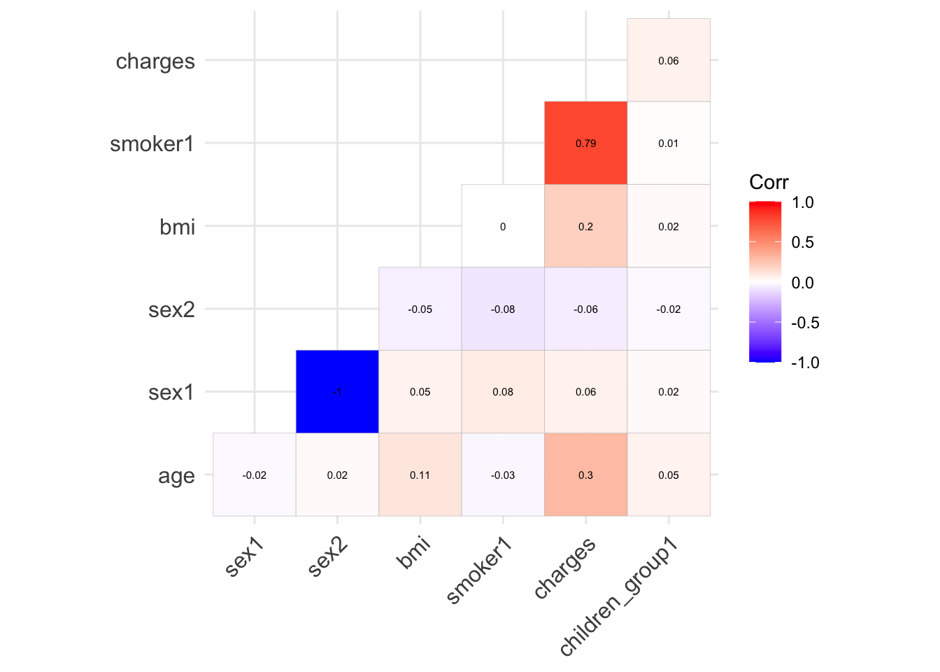
There is no collinearity between any of the variables. Therefore, no need to adjust variable for model building. In addition, smoking seems to be the highest correlated variable to charges among other variables.
Fit regression using all predictors
model <- lm(charges ~ smoker + children_group + sex + age + bmi, data = cost_df)
summary(model)%>%
  broom::tidy() %>%
knitr::kable()| term | estimate | std.error | statistic | p.value |
|---|---|---|---|---|
| (Intercept) | -12225.0034 | 970.40293 | -12.5978633 | 0.0000000 |
| smoker1 | 23822.2843 | 413.01074 | 57.6795754 | 0.0000000 |
| children_group1 | 992.5886 | 336.10888 | 2.9531757 | 0.0032004 |
| sex2 | 123.6608 | 333.73639 | 0.3705345 | 0.7110432 |
| age | 257.8266 | 11.91998 | 21.6297878 | 0.0000000 |
| bmi | 322.2230 | 27.45121 | 11.7380271 | 0.0000000 |
The model building result shows that sex is not a significant variable with p-value < 0.05. Therefore, when we do the stepwise regression, we would likely to remove the variable of sex.
Stepwise regression
step = step(model, direction='both')summary(step)%>%
broom::tidy() %>%
knitr::kable()| term | estimate | std.error | statistic | p.value |
|---|---|---|---|---|
| (Intercept) | -12149.6071 | 948.52261 | -12.808980 | 0.000000 |
| smoker1 | 23810.7572 | 411.70416 | 57.834629 | 0.000000 |
| children_group1 | 990.7412 | 335.96313 | 2.948958 | 0.003244 |
| age | 257.9366 | 11.91243 | 21.652729 | 0.000000 |
| bmi | 321.7303 | 27.41011 | 11.737652 | 0.000000 |
The stepwise regression process confirms that sex is not significant variable. Therefore we remove sex variable and retain all other variables for prediction model.
Final model with significant variables
model1 <- lm(charges ~ smoker + children_group + age + bmi, data = cost_df)
summary(model1) %>%
  broom::tidy() %>%
knitr::kable()| term | estimate | std.error | statistic | p.value |
|---|---|---|---|---|
| (Intercept) | -12149.6071 | 948.52261 | -12.808980 | 0.000000 |
| smoker1 | 23810.7572 | 411.70416 | 57.834629 | 0.000000 |
| children_group1 | 990.7412 | 335.96313 | 2.948958 | 0.003244 |
| age | 257.9366 | 11.91243 | 21.652729 | 0.000000 |
| bmi | 321.7303 | 27.41011 | 11.737652 | 0.000000 |
3. Model diagnostic
par(mfrow = c(2,2))
plot(model1)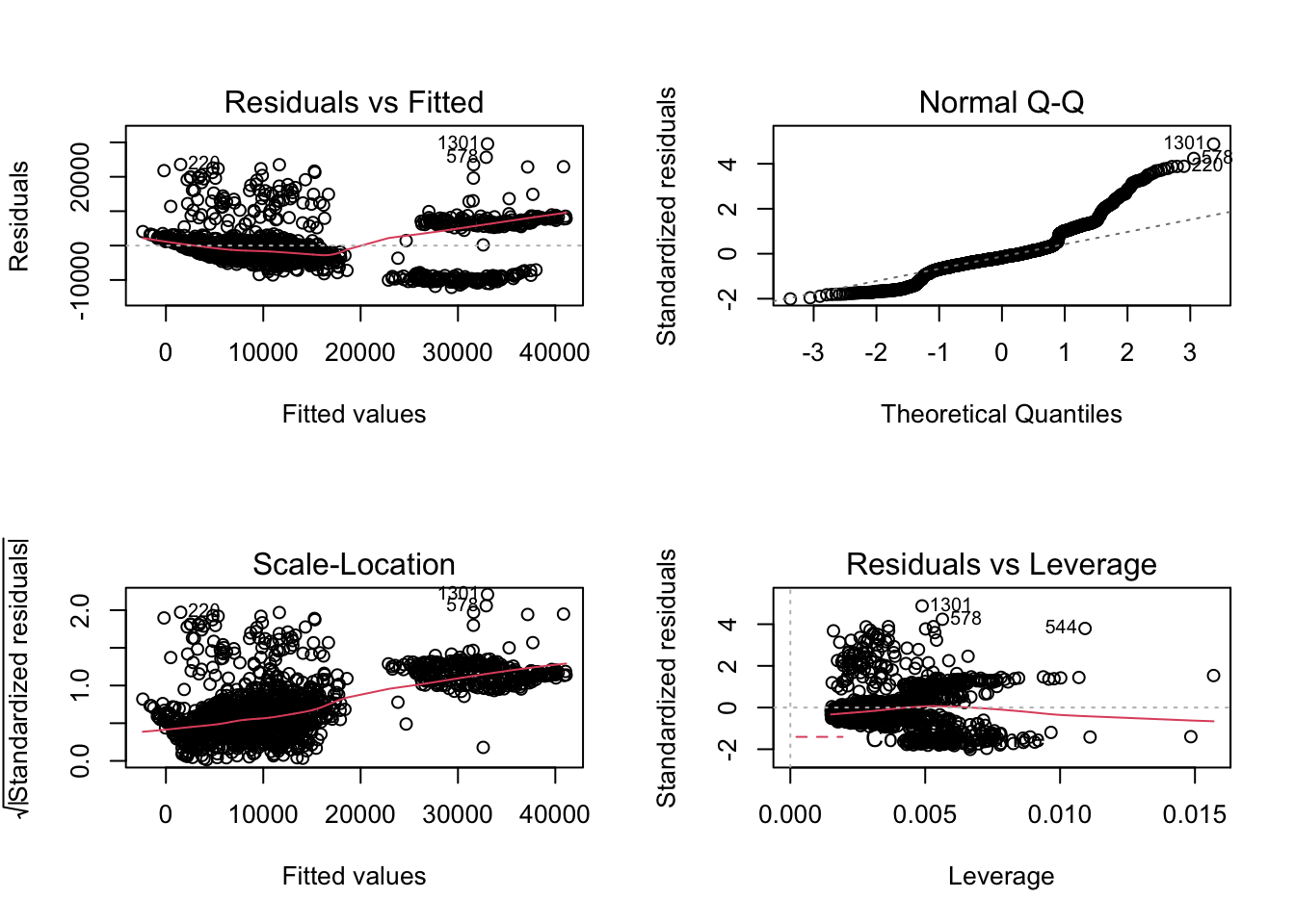
The graph above did not show homoscedasticity of residual. Therefore, we need to transform the model.
4. Model transformation
Box-Cox Transformation
par(mfrow = c(1,2))

boxcox(model1, lambda = seq(-3, 3, by = 0.25))

plot(model1, which = 4) # remove 544, 578, 1301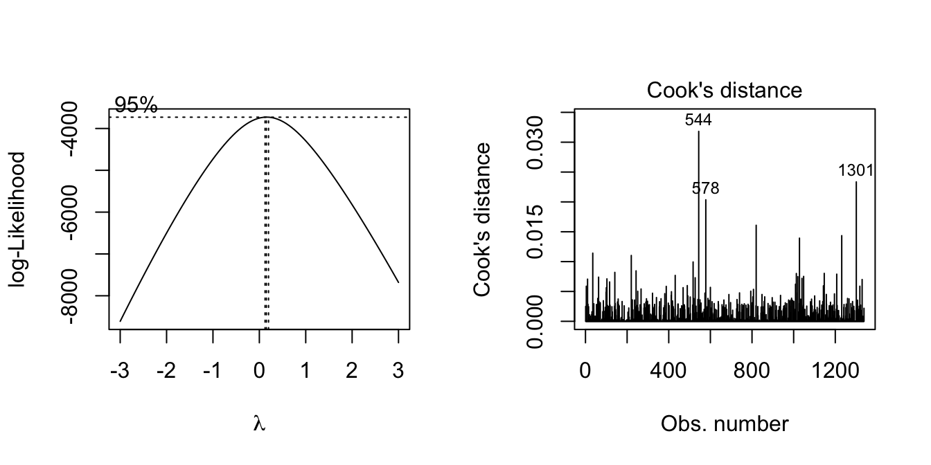
cost_df_out = cost_df[-c(544,578, 1301),]Since lamda = 0, try natural log transformation.
Before transformation, remove outliers first
The outliers are rows 544, 578, 1301. Following model building will use dataset without these outliers.
Transform charges to ln(charges)
#summary(cost_df_out)
cost_df_log = cost_df_out %>%
  mutate(
    Lncharges = log(charges)
  )

# fit multivariate model with log transform
model_log = lm(Lncharges ~ smoker + children_group + age + bmi, data = cost_df_log)
summary(model_log) %>%
  broom::tidy() %>%
knitr::kable()| term | estimate | std.error | statistic | p.value |
|---|---|---|---|---|
| (Intercept) | 6.9709701 | 0.0706776 | 98.630532 | 0e+00 |
| smoker1 | 1.5370576 | 0.0307293 | 50.019359 | 0e+00 |
| children_group1 | 0.2263090 | 0.0250004 | 9.052215 | 0e+00 |
| age | 0.0347807 | 0.0008857 | 39.268460 | 0e+00 |
| bmi | 0.0103985 | 0.0020435 | 5.088614 | 4e-07 |
Above table shows the estimates for each variables when charges is transformed to In(charges).
Diagnostic for transformed model
par(mfrow = c(1,2))

boxcox(model_log)

plot(model_log, which = 1)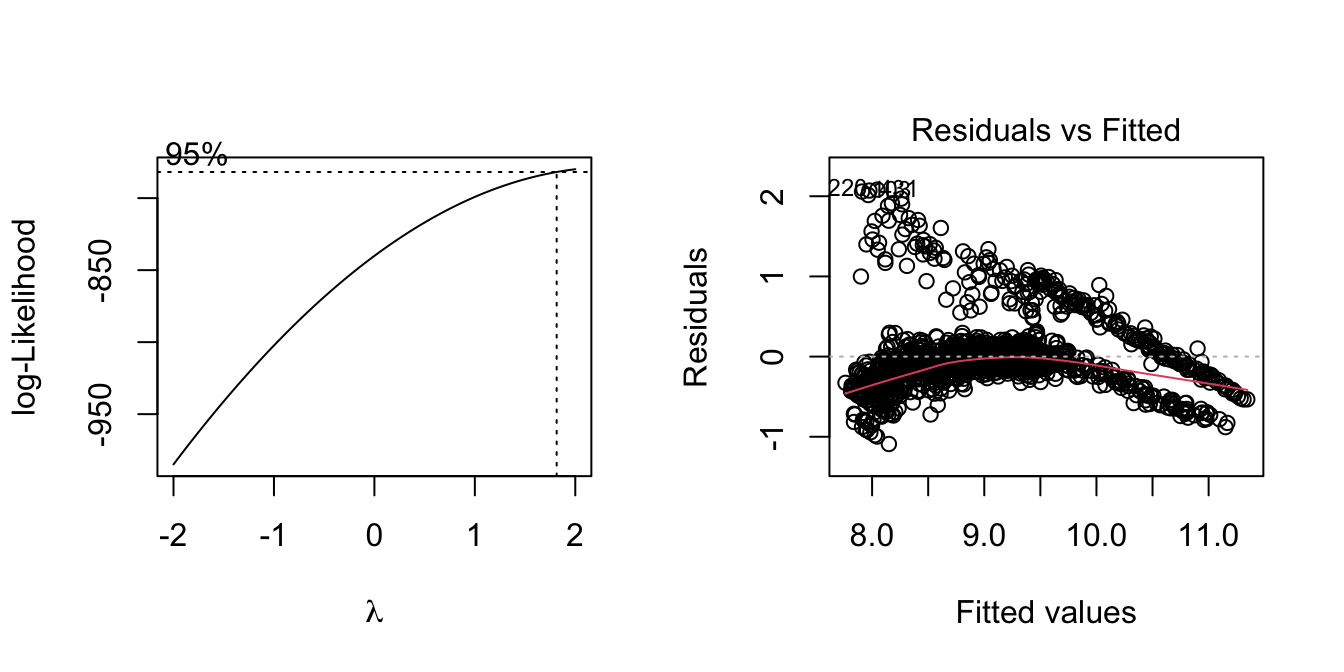
Lamda is near 1 now, and the residual distribution improved from un-transformed data. We conclude this model is acceptable.
Final model
summary(model_log) %>%
  broom::tidy() %>%
knitr::kable()| term | estimate | std.error | statistic | p.value |
|---|---|---|---|---|
| (Intercept) | 6.9709701 | 0.0706776 | 98.630532 | 0e+00 |
| smoker1 | 1.5370576 | 0.0307293 | 50.019359 | 0e+00 |
| children_group1 | 0.2263090 | 0.0250004 | 9.052215 | 0e+00 |
| age | 0.0347807 | 0.0008857 | 39.268460 | 0e+00 |
| bmi | 0.0103985 | 0.0020435 | 5.088614 | 4e-07 |
Decode the model estimates
Holding all other variable constant, smoking is associated with a 155% increase in insurance charges than non-smokers. Being older, higher body mass index, and having at least 1 children also increase insurance charges.